In the following I will demonstrate the basic steps for fitting NMR spectra using ssNake. After you are satisfied with the processing of your dataset you can try to fit the spectrum using a number of built-in functions:

• Lorentian/Gaussian
• CSA
• Quadrupole
• Quadrupole + CSA
• Czjzek
• Czjzek MQMAS
• External (SIMPSON)
• Function

In the following the general fitting procedure is demonstrated on a few example datasets.

Lorentzian / Gaussian Fitting

We start with an already processed 13C{1H} CP-MAS spectrum of a polymer.

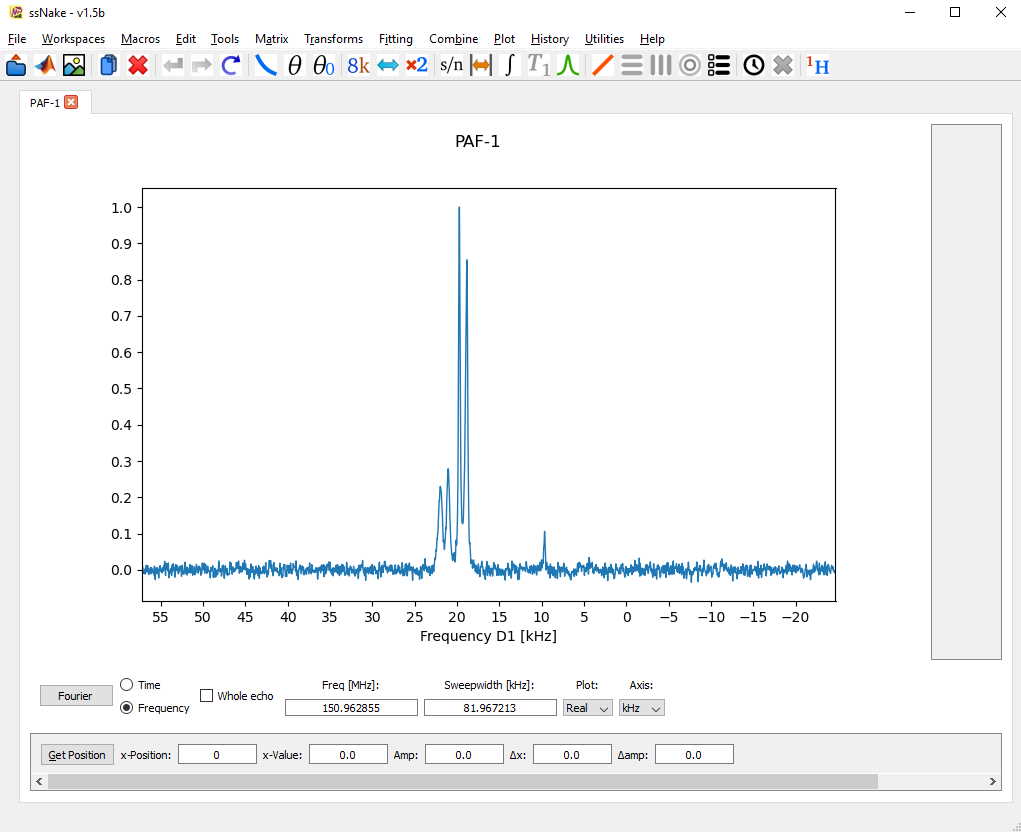
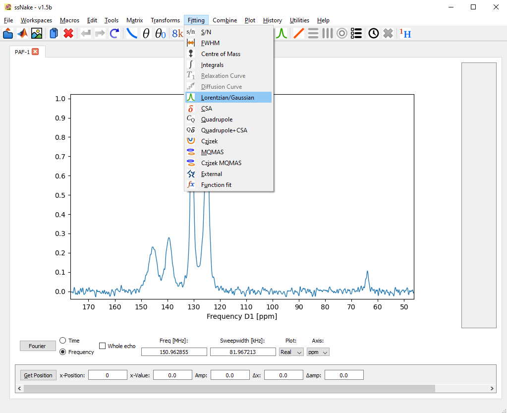
After zooming in and setting the frequency axis to “ppm” we chose the Lorentzian/Gaussian model from the Fitting tab.

We are presented with a new window below our spectrum comprised of two parts. On the left, we find several buttons for simulating the fit model based on the defined parameters (sim), fitting the spectrum (fit) according to the cost function defined in the Preferences tab, functions to copy and export fit parameters and curves (Copy par. and Export/Import) and a functionality to exclude certain spectral regions from the fitting algorithm.

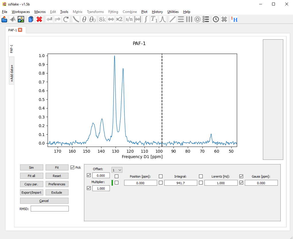
On the right side, we see the currently defined fit components (one currently), defined by position, area (Integral), and Lorentz/Gauss character/width. Additionally, an extra offset and overall lineshape multiplier can be defined, however, I found to use it very little.

While the “pick” tickbox is enabled, lineshape components can be placed in the spectrum through clicking once slightly left of a signal maximum, and a second time slightly right of it. The result is not very convincing, but it helps to quickly place a few lines in the spectrum. Alternatively, the small drop down menu can be set to a different number to add lineshape components.

Here, I have quickly placed five components using the picking tool.

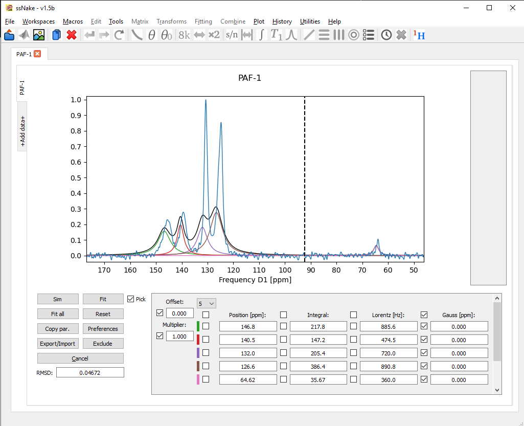
For fitting the spectra, a click on the Fit button is enough. This will try to minimize the root-mean-square-deviation (RMSD, see bottom left) according to the parameters on the right side which are not ticked! To hold a parameter constant it suffices to tick the box next to it. For now I will untick the Gaussian parameter so I will end up with mixed Lorentz/Gaussian components. After a first fit the result looks like this:

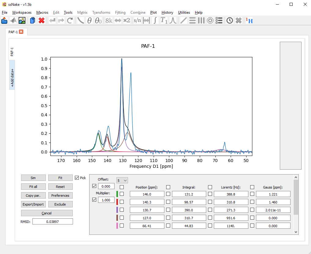
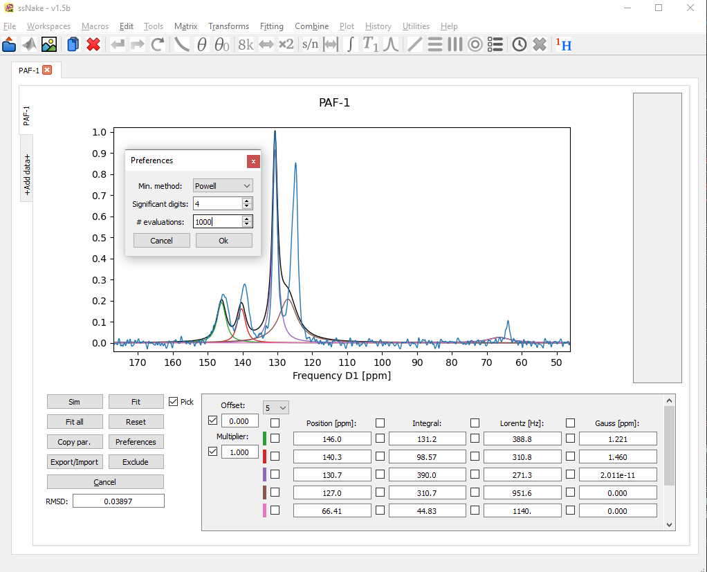
A bit better, but it seems the fitting routine didn’t have enough time to converge on a satisfying result. Using the Preferences tab we can increase the number of iteration steps or “evaluations” to give the fit more time.

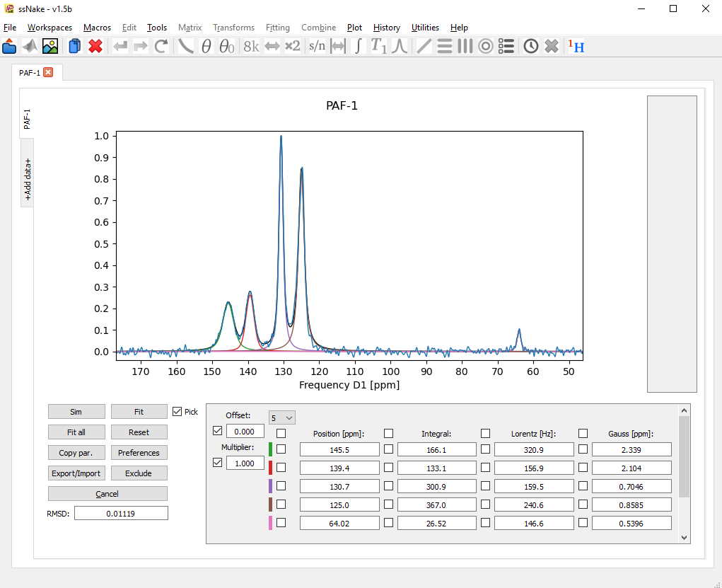
After another round of fitting the result already looks rather solid.

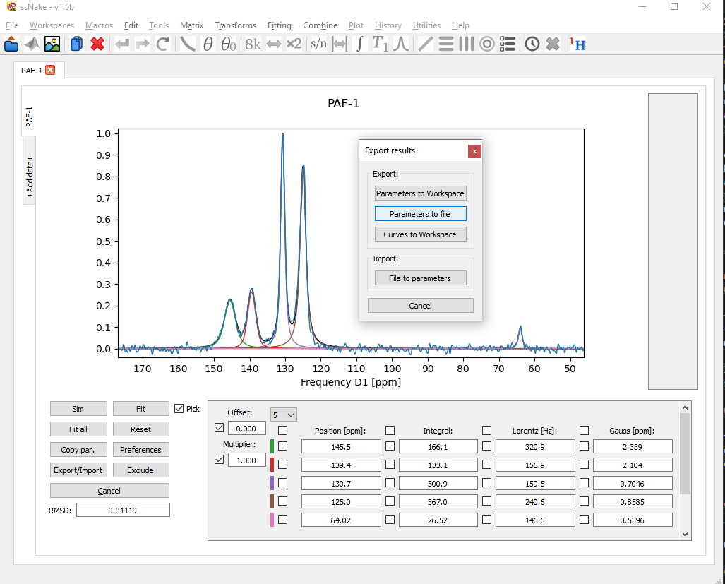
Once I am happy with the result, I can export the fit parameters using the Export/Import tab. For exporting the experimental data and fitted curves together one should use the “Curves to Workspace” button.

After choosing the parts of the data I would like to export, all curves are placed in a new workspace, which I named with the ending “-export”. From here, in order to export the curves to a text file first the axis should be set to ppm, if desired, and then the option under File -> Export -> ASCII (or CSV) needs to be chosen.

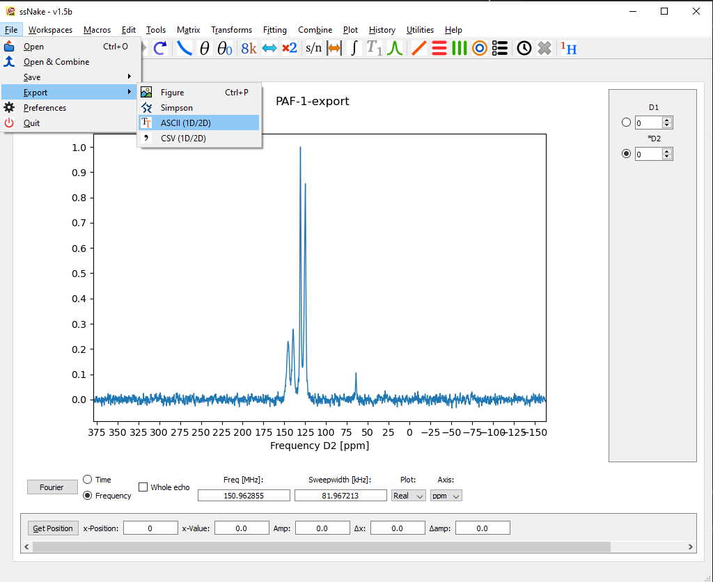
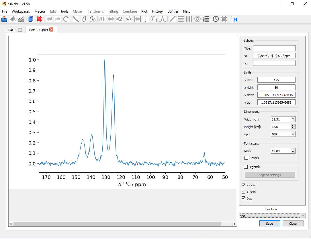
The resulting file can then be imported in other programs for visualization. Alternatively a Figure can be created and exported using ssNake itself, based on the matplotlib package. Therefore, Export -> Figure will open another menu, in which the currently active window can be edited and then saved as different file types.

Czjzek Fitting

Open up the dataset Czjezk_example. Since this data has already been processed in Topspin, we need to only perform a few and sometimes optional steps. First, we do a baseline correction of the dataset (Tools —> Baseline correction), and secondly normalize (Matrix —> Normalize) the spectrum in order to keep the integral values of the fit components in managable sizes.

Once this is done we choose the Czjzek fitting option in the Fitting dropdown menu:

A number of advanced tutorials can be found here.